Example

This tutorial will cover a very practical example of how ror can be applied to some inference pipeline. For this case we will be using the simple Iris dataset from sklearn along with a GMM as our model.

Use ror for more complex problems

ror is a great tool for managing a good seperation of concern in complex inferenece pipelines, however, for very simple problems such as the one presented on this page, it will only add more boiler-plate code which is not worth it for very simple problems.

Creating Schemas

We know that this problem requires three very simple stages; data loading and preprocessing, training/inference, and finally some stage to visualise the results of our model. Based on this, we will be creating our pipeline, but first, we import all the relevant modules for this tutorial.

Module Imports

import matplotlib.pyplot as plt
from sklearn import datasets
from sklearn.mixture import GaussianMixture
from sklearn.decomposition import PCA
from sklearn.preprocessing import StandardScaler

from dataclasses import dataclass
from typing import Tuple

from ror.schemas import BaseSchema
from ror.schemas.fields import field_perishable, field_persistance
from ror.stages import IInitStage, ITerminalStage, IForwardStage
from ror.controlers import BaseController

Then we can define the data schemas. We know that we can simply load the Iris dataset from sklearn, and we should standardise the dataset, so we account for this in our data schemas.

Data Schemas

@dataclass
class InitStageInput(BaseSchema):
    data: object = field_perishable()

@dataclass
class InitStageOutput(BaseSchema):
    X_pca: object = field_persistance()
    X_std: object = field_perishable()
    model: object = field_persistance()

@dataclass
class InferenceStageOutput(BaseSchema):
    X_pca: object = field_perishable()
    model: object = field_perishable()
    labels: object = field_persistance()

@dataclass
class VisStageOutput(BaseSchema):
    labels: object = field_persistance()

Note that we set some fields to be perishable, which prevents this data from being propagated through to the next stages and we can simply ignore them after they have served their purpose. Additionally, we have the X_pca field such that we can visualise the data at the end along two principal components.

Linking Stages

Based on these schemas we allready have a decent idea of how we should link the stages, and we can do this very simply using the provided interfaces from ror.

Defining Stages

class VisStage(ITerminalStage[InferenceStageOutput, VisStageOutput]):
    def compute(self) -> None:
        # Visualize the clusters
        plt.figure(figsize=(8, 6))
        colors = ['r', 'g', 'b']

        for i in range(3):
            plt.scatter(
                self.input.X_pca[self.input.labels == i, 0],
                self.input.X_pca[self.input.labels == i, 1],
                color=colors[i],
                label=f'Cluster {i+1}'
            )

        plt.title('Gaussian Mixture Model Clustering')
        plt.xlabel('Principal Component 1')
        plt.ylabel('Principal Component 2')
        plt.legend()
        plt.show()

        self._output = self.input.get_carry()

    def get_output(self) -> VisStageOutput:
        return VisStageOutput(**self._output)

class InferenceStage(IForwardStage[InitStageOutput, InferenceStageOutput, VisStage]):
    def compute(self) -> None:
        # Fit Guassian mixture to dataset
        self.input.model.fit(self.input.X_std)

        # Predict the labels
        labels = self.input.model.predict(self.input.X_std)

        self._output = {
            "labels": labels,
            **self.input.get_carry()
        }

    def get_output(self) -> Tuple[VisStage, InferenceStageOutput]:
        return VisStage(), InferenceStageOutput(**self._output)


class InitStage(IInitStage[InitStageInput, InitStageOutput, InferenceStage]):
    def compute(self) -> None:
        # Load the dataset
        X = self.input.data.data

        # Standardize the features
        scaler = StandardScaler()
        X_std = scaler.fit_transform(X)

        # Apply PCA to reduce dimensionality for visualization
        pca = PCA(n_components=2)
        X_pca = pca.fit_transform(X_std)

        # Fit a Gaussian Mixture Model
        gmm = GaussianMixture(n_components=3, random_state=42)

        self._output = {
            "X_pca": X_pca,
            "X_std": X_std,
            "model": gmm,
            **self.input.get_carry()
        }

    def get_output(self) -> Tuple[InferenceStage, InitStageOutput]:
        return InferenceStage(), InitStageOutput(**self._output)

Note that we define the stages in reverse order, this is just so that we can have the intermediate references between stages. However, in a production setting the schemas and stages should be seperated into different files which will make the code easier to maintain. When we then define the controller with some input data, we can run the discover method to observe how our stages were linked.

Defining Pipeline Controller

iris = datasets.load_iris()

input_data = InitStageInput(data=iris)
controller = BaseController(init_data=input_data, init_stage=InitStage)
controller.discover()

Below you can see an example of the expected output when running the discover method on this pipeline.

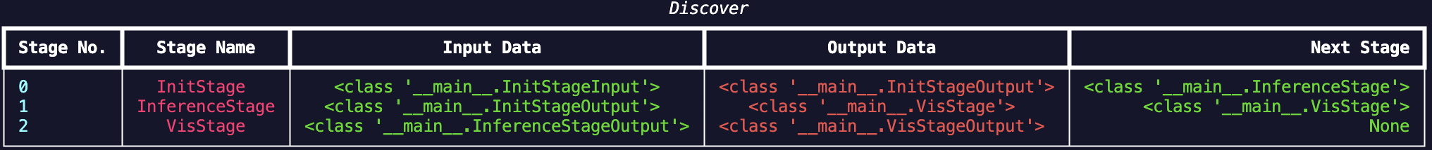
Output of running the discover method of the controller for the above pipeline.

Running the Pipeline

Given that we have allready defined the controller with some input data. We can simply run the start method of the controller to get the output and the final visualisation of the predictions for the GMM.

Running the Pipeline

iris = datasets.load_iris()

output, run_id = controller.start()

With this we should get the following output.

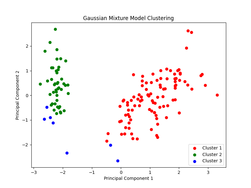
Visualisation of the results from our GMM model defined with ror.

Congratulations you defined your first ror! As mentioned above this library is meant for more complex inference pipelines, however, I hope this served as a gentle introduction into how ror works.